Machine Learning
Supervised Learning - Softmax Classification (multi-variable 1)
emilia park
2023. 8. 6. 20:41
728x90
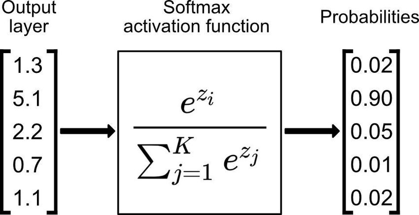
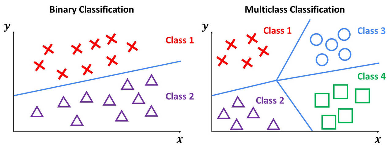
Softmax Classifiation : 주어진 입력에 따라 3개 이상의 class에서의 예측
(=Multi Classification)
Linear : H(x) ∈ (-inf, inf)
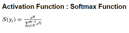
Softmax : H(x) ∈ [0,1]
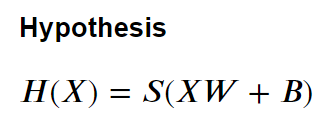
Step1) Hypothesis
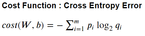
Step2) Cost function
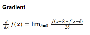
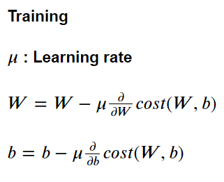
Step3) Training - gradient descent method
Numpy
w/o min-max scaling
#load module
import numpy as np
import matplotlib.pyplot as plt
#input & label
x_input = np.array([[1, 1], [2, 2.5], [2.5, 1.3], [4.3, 9.5],
                    [5.5, 7.0], [6, 8.2], [7, 5], [8, 6], [9, 4.5]], dtype=np.float32)
labels = np.array([[1, 0, 0], [1, 0, 0], [1, 0, 0], [0, 1, 0], [0, 1, 0],
                   [0, 1, 0], [0, 0, 1], [0, 0, 1], [0, 0, 1]], dtype=np.float32)

#weight and bias
n_var, n_class = 2, 3
W = np.random.normal(size=(n_var, n_class))
B = np.random.normal(size=(n_class,))
#Function Generation
def Softmax(y):
    c = np.max(y, axis = 1)
    c = c.reshape((-1,1))
    exp_y = np.exp(y-c)

    sum_exp_y = np.sum(exp_y, axis = 1)
    sum_exp_y = sum_exp_y.reshape((-1,1))

    res_y = exp_y/sum_exp_y

    return res_y

def Hypothesis(x):
    return Softmax(np.matmul(x, W) + B)

def Cost():
    return np.mean(-np.sum(labels * np.log(Hypothesis(x_input)),axis=1))

def Gradient():
    global W, B
    delta = 5e-7

    #W gradient
    pres_W = W.copy()
    grad_W = np.zeros_like(W)

    for i in range(W.shape[0]):
        for j in range(W.shape[1]):
            W[i,j] = pres_W[i,j] + delta
            cost_p = Cost()
            W[i,j] = pres_W[i,j] - delta
            cost_m = Cost()

            grad_W[i,j] = (cost_p - cost_m)/(2*delta)
            W[i,j] = pres_W[i,j]

    #B gradient
    pres_B = B.copy()
    grad_B = np.zeros_like(B)

    for i in range(B.size):
        B[i] = pres_B[i] + delta
        cost_p = Cost()
        B[i] = pres_B[i] - delta
        cost_m = Cost()

        grad_B[i] = (cost_p-cost_m)/(2*delta)
        B[i] = pres_B[i]

    return grad_W, grad_B
#Parameter
epochs = 10000
lr = 0.5

training_idx = np.arange(0, epochs+1, 1)
cost_graph = np.zeros(epochs+1)


#Training
for cnt in range(0, epochs+1):
    cost_graph[cnt] = Cost()
    if cnt % (epochs//5) == 0:
        print("[Epochs : {:>6}] Cost = {:>10.4}".format(cnt, cost_graph[cnt]))
        print("W = {:}".format(W))
        print("B = {:}".format(B))


    grad_W, grad_B = Gradient()
    W -= lr * grad_W
    B -= lr * grad_B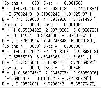
#Prediction (using input value)
test_set = np.array([[0.1, 3], [4.7, 9], [9, 1.5]])
Hx = Hypothesis(test_set)
H = np.argmax(Hx, axis = 1)
for i in range(test_set.shape[0]):
    print("Input : {} => Group : {} , Pred : {}".format(test_set[i], H[i], Hx[i]))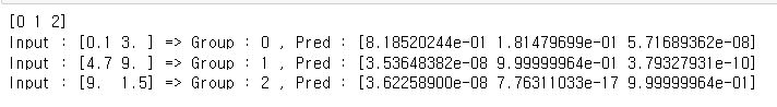
#Cost function graph
plt.title("'Cost / Epochs' Graph")
plt.xlabel("Epochs")
plt.ylabel("Cost")
plt.plot(training_idx, cost_graph)
plt.xlim(0, epochs)
plt.grid(True)
plt.semilogy()
plt.show()
Tensorflow
w/o min-max scaling
#load module
import numpy as np
import tensorflow as tf
import matplotlib.pyplot as plt
#input & label
x_input = tf.constant([[1, 1], [2, 2.5], [2.5, 1.3], [4.3, 9.5],
                    [5.5, 7.0], [6, 8.2], [7, 5], [8, 6], [9, 4.5]], dtype=tf.float32)
labels = tf.constant([[1, 0, 0], [1, 0, 0], [1, 0, 0], [0, 1, 0], [0, 1, 0],
                   [0, 1, 0], [0, 0, 1], [0, 0, 1], [0, 0, 1]], dtype=tf.float32)

#weight and bias
n_var, n_class = 2, 3
W = tf.Variable(tf.random.normal((n_var, n_class),dtype=tf.float32))
B = tf.Variable(tf.random.normal((n_class,),dtype=tf.float32))
#Function Generation
def logits(x):
    return tf.matmul(x,W) + B

def Hypothesis(x):
    return tf.nn.softmax(logits(x))

def Cost():
    logit_value = logits(x_input)
    return tf.reduce_mean(tf.nn.softmax_cross_entropy_with_logits(logits=logit_value, labels=labels))
#Parameter
epochs = 10000
lr = 0.5
opt = tf.keras.optimizers.SGD(learning_rate = lr)

training_idx = np.arange(0, epochs+1, 1)
cost_graph = np.zeros(epochs+1)


#Training
for cnt in range(0, epochs+1):
    cost_graph[cnt] = Cost()
    if cnt % (epochs//5) == 0:
        print("[Epochs : {:>6}] Cost = {:>10.4}".format(cnt, cost_graph[cnt]))
        print("W = {:}".format(W.numpy()))
        print("B = {:}".format(B.numpy()))

    opt.minimize(Cost, [W,B])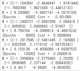
#Prediction (using input value)
test_set = tf.constant([[0.1, 3], [4.7, 9], [9.0, 5.0]], dtype = tf.float32)
Hx = Hypothesis(test_set)
H = np.argmax(Hx, axis = 1)

for i in range(test_set.shape[0]):
    print("Input : {} => Group : {} , Pred : {}".format(test_set[i], H[i], Hx[i]))
#Cost function graph
plt.title("'Cost / Epochs' Graph")
plt.xlabel("Epochs")
plt.ylabel("Cost")
plt.plot(training_idx, cost_graph)
plt.xlim(0, epochs)
plt.grid(True)
plt.semilogy()
plt.show()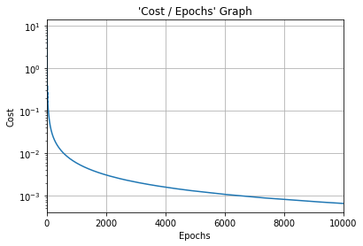
728x90